FOCUS: Fdtd On CUda Simulator

The Finite Difference in the Time Domain (FDTD) is a numerical technique commonly used in electromagnetics to solve complex problems where, due to the complexity of the geometries and/or of the dielectric properties of the materials located inside the simulation scenario, an analytical solution cannot be found. Finding an analytical solution for a complex problem, in fact, usually requires the introduction of strong simplifications, that can make the final results unusable.

Principal investigator: Dott. Gaetano Bellanca gaetano.bellanca@unife.it
Collaborators: Matteo Ruina
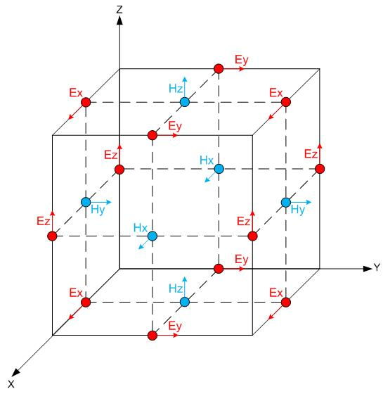
The FDTD technique solves the Maxwell’s curl equations directly in the time domain by replacing the differential operators (for both time and space variables) with finite differences expressions. This is the first approximation of the FDTD technique. For this reason, a discretization of both time and 3D space axes is introduced. The computational domain (usually in 3D) is therefore represented with a properly defined mesh; the fundamental element of the mesh is the elementary cell, where the six components of the electromagnetic (e.m.) field (Ex, Ey and Ez, Hx, Hy and Hz respectively) are calculated iteratively. Each cell is filled with the dielectric properties of the material located in the corresponding point of the simulated scenario. As a consequence, the physical domain is represented with a discrete set of cells. This is the second approximation (staircase approximation of the geometry) of the FDTD method. The use of a ‘staggered grid’ (in which the field components are positioned in different points inside the elementary cell) and the possibility to interplay the calculation of the electric and magnetic fields results in a ‘leapfrog’ algorithm which allows the iterative solution (time evolution of the e.m. fields) in explicit form, thus avoiding any matrix inversion procedure.

Fig. 1: Yee Cell with position of each field component.

The core algorithm is very simple and consists of a six vector loops, which perform the update of each component of the electric and magnetic field respectively in every point of the grid. Unfortunately, FDTD is quiet demanding in terms of computational resources as it requires a very small (ranging from 1/10 to 1/20) pitch of the mesh respect to the wavelength of the considered e.m. radiation. Moreover, the temporal time step cannot be chosen independently from the mesh size, but must be selected in order to guarantee the stability of the algorithm (Courant stability). In practice, to solve problems corresponding to realistic scenarios (3D domains with dimensions of the order of some wavelengths for each side), a large amount of memory (to represents all the cells of the mesh) and a large amount of time-steps (to eliminate the transients of the field excitation) are needed. As a consequence, parallelization of the code is often used.

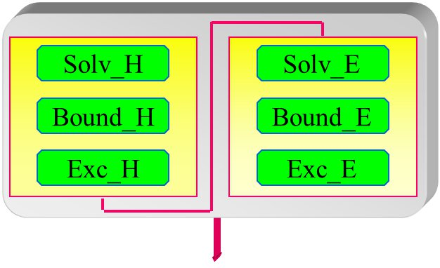
Fig. 2: core algorithm of the FDTD code.

The simple and explicit nature of the algorithm can take full advantage of the features of a parallel computer as a single field component (say e_x) can be evaluated, in a fixed time-step and in each point of the mesh, by using only its previous value in the same point and the field components (say h_y and h_z) in the closest cells of the mesh and in the previous time-step. Therefore, all the unknowns are calculated using known variables, thus making all the computations very fast as no matrix inversion is needed. The Message Passing Interface (MPI) library can be used to efficiently manage all the procedures needed to synchronize the activities of the nodes of the system (PEs) during the parallel execution of a simulation.
The Optics Group of the Department of Engineering has developed many years ago a 3D-FDTD code based on MPI paradigm for the parallelization, which is actually used in the framework of different research projects.
This code is written in Fortran 90 and scales very well on parallel clusters. Unfortunately, the same scalability is not obtained on multicore processors, due to the limitation on the bandwidth for the access of the data into the memory of each node, which is shared between the different cores.

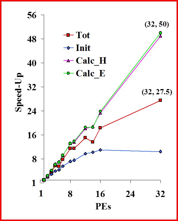
Fig. 3: scaling performance of the UniFE's 3D-FDTD code on the ORIGIN 2000 of Cineca. An overall speed up of 27.5 with 32 processors is reported

The aim of this project is the optimization of a computational kernel for e.m. field calculation based on the FDTD algorithm on GPU architectures. The idea is to use two levels for the parallelization:

1. MPI level, to distribute the huge computational domain (usually the number of points of the mesh range from 30×10⁶ to 50×10⁶) between the processors of the computation nodes;
2. CUDA level, to speed-up the computation on each node of the system, where only a small portion of the overall domain has been loaded.

CUDA optimization of the solving algorithm for the e.m. field will be managed first, to avoid problems in debugging of the code of the complete simulator. Once optimized the core of the algorithm, the new CUDA kernel will be included in the 3D-FDTD simulator. Due to the fact that the partition of the simulated scenario with MPI creates local data on each node, performance degradation determined by mixing of the two parallelization paradigms is not expected.