Outline

• Logic

• Probabilistic logics

• Probabilistic logic programming

• Applications

• Inference

• Learning

• Examples

Logic

• Useful to model domains with complex relationships among entities

• Various forms:

  • First Order Logic

  • Logic Programming

  • Description Logics

First Order Logic

• Very expressive

• Open World Assumption

• Undecidable

\[\begin{array}{l} \forall x\ Intelligent(x)\rightarrow GoodMarks(x)\\ \forall x,y\ Friends(x,y)\rightarrow (Intelligent(x)\leftrightarrow Intelligent(y)) \end{array}\]

Logic Programming

• A subset of First Order Logic

• Closed World Assumption

• Turing complete

• Prolog

\[\begin{array}{l} \mathit{flu}(bob).\\ hay\_\mathit{fever}(bob).\\ sneezing(X)\leftarrow \mathit{flu}(X).\\ sneezing(X)\leftarrow hay\_\mathit{fever}(X).\\ \end{array}\]

Description Logics

• Subsets of First Order Logic

• Open World Assumption

• Decidable, efficient inference

• Special syntax using concepts (unary predicates) and roles (binary predicates)

\[\begin{aligned} &&{\mathit{fluffy}}: Cat\\ &&tom : Cat \\ &&Cat \sqsubseteq Pet \\ &&\exists hasAnimal.Pet \sqsubseteq NatureLover\\ &&(kevin, {\mathit{fluffy}}):hasAnimal \\ &&(kevin, tom):hasAnimal \end{aligned}\]

Combining Logic and Probability

• Logic does not handle well uncertainty

• Graphical models do not handle well relationships among entities

• Solution: combine the two

• Many approaches proposed in the areas of Logic Programming, Uncertainty in AI, Machine Learning, Databases, Knowledge Representation

Probabilistic Logic Programming

• Distribution Semantics [Sato ICLP95]

• A probabilistic logic program defines a probability distribution over normal logic programs (called instances or possible worlds or simply worlds)

• The distribution is extended to a joint distribution over worlds and interpretations (or queries)

• The probability of a query is obtained from this distribution

Probabilistic Logic Programming (PLP) Languages under the Distribution Semantics

• Probabilistic Logic Programs [Dantsin RCLP91]

• Probabilistic Horn Abduction [Poole NGC93], Independent Choice Logic (ICL) [Poole AI97]

• PRISM [Sato ICLP95]

• Logic Programs with Annotated Disjunctions (LPADs) [Vennekens et al. ICLP04]

• ProbLog [De Raedt et al. IJCAI07]

• They differ in the way they define the distribution over logic programs

PRISM

\[\begin{array}{l} sneezing(X)\leftarrow \mathit{flu}(X), msw(\mathit{flu}\_sneezing(X),1).\\ sneezing(X)\leftarrow hay\_\mathit{fever}(X),msw(hay\_\mathit{fever}\_sneezing(X),1).\\ \mathit{flu}(bob).\\ hay\_\mathit{fever}(bob).\\ \\ values(\mathit{flu}\_sneezing(\_X),[1,0]).\\ values(hay\_\mathit{fever}\_sneezing(\_X),[1,0]).\\ :- set\_sw(\mathit{flu}\_sneezing(\_X),[0.7,0.3]).\\ :- set\_sw(hay\_\mathit{fever}\_sneezing(\_X),[0.8,0.2]). \end{array}\]

• Distributions over \(msw\) facts (random switches)

• Worlds obtained by selecting one value for every grounding of each \(msw\) statement

Logic Programs with Annotated Disjunctions

\[\begin{array}{l} sneezing(X):0.7\vee null:0.3\leftarrow \mathit{flu}(X).\\ sneezing(X):0.8\vee null:0.2\leftarrow hay\_\mathit{fever}(X).\\ \mathit{flu}(bob).\\ hay\_\mathit{fever}(bob).\\ \end{array}\]

• Distributions over the head of rules

• \(null\) does not appear in the body of any rule

• Worlds obtained by selecting one atom from the head of every grounding of each clause

ProbLog

\[\begin{array}{l} sneezing(X)\leftarrow \mathit{flu}(X),\mathit{flu}\_sneezing(X).\\ sneezing(X)\leftarrow hay\_\mathit{fever}(X),hay\_\mathit{fever}\_sneezing(X).\\ \mathit{flu}(bob).\\ hay\_\mathit{fever}(bob).\\ 0.7::\mathit{flu}\_sneezing(X).\\ 0.8::hay\_\mathit{fever}\_sneezing(X).\\ \end{array}\]

• Distributions over facts

• Worlds obtained by selecting or not every grounding of each probabilistic fact

Distribution Semantics

• Case of no function symbols: finite Herbrand universe, finite set of groundings of each switch/clause

• Atomic choice: selection of the \(i\)-th atom for grounding \(C\theta\) of switch/clause \(C\)

  • represented with the triple \((C,\theta,i)\)

  • a ProbLog fact \(p::F\) is interpreted as \(F:p\vee null:1-p.\)

• Example \(C_1=sneezing(X):0.7\vee null:0.3\leftarrow \mathit{flu}(X).\), \((C_1,\{X/bob\},1)\)

• Composite choice \(\kappa\): consistent set of atomic choices

• The probability of composite choice \(\kappa\) is \[P(\kappa)=\prod_{(C,\theta,i)\in \kappa}P_0(C,i)\]

Distribution Semantics

• Selection \(\sigma\): a total composite choice (one atomic choice for every grounding of each clause)

• A selection \(\sigma\) identifies a logic program \(w_\sigma\) called world

• The probability of \(w_\sigma\) is \(P(w_\sigma)=P(\sigma)=\prod_{(C,\theta,i)\in \sigma}P_0(C,i)\)

• Finite set of worlds: \(W_T=\{w_1,\ldots,w_m\}\)

• \(P(w)\) distribution over worlds: \(\sum_{w\in W_T}P(w)=1\)

Distribution Semantics

• Ground query \(Q\)

• \(P(Q|w)=1\) if \(Q\) is true in \(w\) and 0 otherwise

• \(P(Q)=\sum_{w}P(Q,w)=\sum_{w}P(Q|w)P(w)=\sum_{w\models Q}P(w)\)

Example Program (LPAD) Worlds

\[\begin{array}{ll} sneezing(bob)\leftarrow \mathit{flu}(bob).& null\leftarrow \mathit{flu}(bob).\\ sneezing(bob)\leftarrow hay\_\mathit{fever}(bob).& sneezing(bob)\leftarrow hay\_\mathit{fever}(bob).\\ \mathit{flu}(bob).&\mathit{flu}(bob).\\ hay\_\mathit{fever}(bob).&hay\_\mathit{fever}(bob).\\ P(w_1)=0.7\times 0.8 &P(w_2)=0.3\times 0.8\\ \\ sneezing(bob)\leftarrow \mathit{flu}(bob).& null\leftarrow \mathit{flu}(bob).\\ null\leftarrow hay\_\mathit{fever}(bob).& null\leftarrow hay\_\mathit{fever}(bob).\\ \mathit{flu}(bob).&\mathit{flu}(bob).\\ hay\_\mathit{fever}(bob). &hay\_\mathit{fever}(bob).\\ P(w_3)=0.7\times 0.2 &P(w_4)=0.3\times 0.2 \end{array}\] \[\label{ds} P(Q)=\sum_{w\in W_\mathcal{T}}P(Q,w)=\sum_{w \in W_\mathcal{T}}P(Q|w)P(w)=\sum_{w\in W_\mathcal{T}: w\models Q}P(w)\]

• \(sneezing(bob)\) is true in 3 worlds

• \(P(sneezing(bob))=0.7\times 0.8+0.3\times 0.8+0.7\times 0.2=0.94\)

Example Program (ProbLog) Worlds

• 4 worlds

\[\begin{array}{l} sneezing(X)\leftarrow \mathit{flu}(X),\mathit{flu}\_sneezing(X).\\ sneezing(X)\leftarrow hay\_\mathit{fever}(X),hay\_\mathit{fever}\_sneezing(X).\\ \mathit{flu}(bob).\\ hay\_\mathit{fever}(bob). \end{array}\]

\[\begin{array}{ll} \mathit{flu}\_sneezing(bob).\\ hay\_\mathit{fever}\_sneezing(bob).&hay\_\mathit{fever}\_sneezing(bob).\\ P(w_1)=0.7\times 0.8 &P(w_2)=0.3\times 0.8\\ \mathit{flu}\_sneezing(bob).\\ P(w_3)=0.7\times 0.2 &P(w_4)=0.3\times 0.2 \end{array}\]

• \(sneezing(bob)\) is true in 3 worlds

• \(P(sneezing(bob))=0.7\times 0.8+0.3\times 0.8+0.7\times 0.2=0.94\)

Logic Programs with Annotated Disjunctions

\[\begin{array}{l} strong\_sneezing(X):0.3\vee moderate\_sneezing(X):0.5\leftarrow \mathit{flu}(X).\\ strong\_sneezing(X):0.2\vee moderate\_sneezing(X):0.6\leftarrow hay\_\mathit{fever}(X).\\ \mathit{flu}(bob).\\ hay\_\mathit{fever}(bob).\\ \end{array}\]

• 9 worlds

• \(P(strong\_sneezing(bob))=?\)

Examples

Throwing coins

heads(Coin):1/2 ; tails(Coin):1/2 :-
  toss(Coin),\+biased(Coin).
heads(Coin):0.6 ; tails(Coin):0.4 :-
  toss(Coin),biased(Coin).
fair(Coin):0.9 ; biased(Coin):0.1.
toss(coin).

Russian roulette with two guns

death:1/6 :- pull_trigger(left_gun).
death:1/6 :- pull_trigger(right_gun).
pull_trigger(left_gun).
pull_trigger(right_gun).

Examples

Mendel’s inheritance rules for pea plants

color(X,purple):-cg(X,_A,p).
color(X,white):-cg(X,1,w),cg(X,2,w).
cg(X,1,A):0.5 ; cg(X,1,B):0.5 :- 
  mother(Y,X),cg(Y,1,A),cg(Y,2,B). 
cg(X,2,A):0.5 ; cg(X,2,B):0.5 :- 
  father(Y,X),cg(Y,1,A),cg(Y,2,B).

Probability of paths

path(X,X).
path(X,Y):-path(X,Z),edge(Z,Y).
edge(a,b):0.3.
edge(b,c):0.2.
edge(a,c):0.6.

Encoding Bayesian Networks

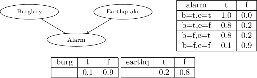
burg(t):0.1 ; burg(f):0.9.
earthq(t):0.2 ; earthq(f):0.8.
alarm(t):-burg(t),earthq(t).
alarm(t):0.8 ; alarm(f):0.2:-burg(t),earthq(f).
alarm(t):0.8 ; alarm(f):0.2:-burg(f),earthq(t).
alarm(t):0.1 ; alarm(f):0.9:-burg(f),earthq(f).

PLP Online

• http://cplint.lamping.unife.it/

  • Inference (knwoledge compilation, Monte Carlo)

  • Parameter learning (EMBLEM)

  • Structure learning (SLIPCOVER)

• https://dtai.cs.kuleuven.be/problog/

  • Inference (knwoledge compilation, Monte Carlo)

  • Parameter learning (LFI-ProbLog)

Monty Hall Puzzle

• A player is given the opportunity to select one of three closed doors, behind one of which there is a prize.

• Behind the other two doors are empty rooms.

• Once the player has made a selection, Monty is obligated to open one of the remaining closed doors which does not contain the prize, showing that the room behind it is empty.

• He then asks the player if he would like to switch his selection to the other unopened door, or stay with his original choice.

• Does it matter if he switches?

Monty Hall Puzzle

:- use_module(library(pita)).
:- endif. 
:- pita. 
:- begin_lpad.
prize(1):1/3; prize(2):1/3; prize(3):1/3.
selected(1).
open_door(A):0.5; open_door(B):0.5:- 
  member(A,[1,2,3]), member(B,[1,2,3]),
  A<B, \+ prize(A), \+ prize(B),
  \+ selected(A), \+ selected(B).
open_door(A):-
  member(A,[1,2,3]), \+ prize(A),
  \+ selected(A), member(B,[1,2,3]),
  prize(B), \+ selected(B).
win_keep:- 
  selected(A), prize(A).
win_switch:- 
  member(A,[1,2,3]),
  \+ selected(A), prize(A), 
  \+ open_door(A).
:- end_lpad.

Monty Hall Puzzle

• Queries:

prob(win_keep,Prob).
prob(win_switch,Prob).

Expressive Power

• All languages under the distribution semantics have the same expressive power

• LPADs have the most general syntax

• There are transformations that can convert each one into the others

• PRISM, ProbLog to LPAD: direct mapping

LPADs to ProbLog

• Clause \(C_i\) with variables \(\overline{X}\) \[H_1:p_1 \vee\ldots\vee H_n:p_n \leftarrow B.\] is translated into \[\begin{array}{l} H_1\leftarrow B,f_{i,1}(\overline{X}).\\ H_2\leftarrow B,not( f_{i,1}(\overline{X})),f_{i,2}(\overline{X}).\\ \vdots\\ H_n\leftarrow B,not(f_{i,1}(\overline{X})),\ldots,not( f_{i,n-1}(\overline{X})).\\ \pi_1::f_{i,1}(\overline{X}).\\ \vdots\\ \pi_{n-1}::f_{i,n-1}(\overline{X}). \end{array}\] where \(\pi_1=p_1\), \(\pi_2=\frac{p_2}{1-\pi_1}\), \(\pi_3=\frac{p_3}{(1-\pi_1)(1-\pi_2)},\ldots\)

• In general \(\pi_i=\frac{p_i}{\prod_{j=1}^{i-1}(1-\pi_j)}\)

Conversion to Bayesian Networks

• PLP can be converted to Bayesian networks

• Conversion for an LPAD \(T\)

• For each atom \(A\) in \(H_T\) a binary variable \(A\)

• For each clause \(C_i\) in the grounding of \(T\)

  \[H_1:p_1 \vee \ldots\vee H_n:p_n \leftarrow B_1, \ldots B_m,\neg {C_1},\ldots,\neg {C_l}\] a variable \(CH_i\) with \(B_1,\ldots,B_m,C_1,\ldots,C_l\) as parents and \(H_1\), \(\ldots\), \(H_n\) and \(null\) as values

Conversion to Bayesian Networks

• \[H_1:p_1 \vee \ldots\vee H_n:p_n \leftarrow B_1, \ldots B_m,\neg {C_1},\ldots,\neg {C_l}\]

• The CPT of \(CH_i\) is

Conversion to Bayesian Networks

• Each variable \(A\) corresponding to atom \({A}\) has as parents all the variables \(CH_i\) of clauses \(C_i\) that have \({A}\) in the head.

• The CPT for \(A\) is:

Conversion to Bayesian Networks

\( \begin{array}{lll} C_1&=&{x1} :0.4\vee {x2}:0.6.\\ C_2&=&{x2}:0.1 \vee {x3}:0.9.\\ C_3&=&{x4}:0.6\vee {x5}:0.4\leftarrow {x1}.\\ C_4&=& {x5}:0.4\leftarrow {x2},{x3}.\\ C_5&=& {x6}:0.3 \vee {x7}:0.2\leftarrow {x2},{x5}. \end{array}\)

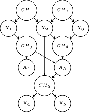
Conversion to Bayesian Networks

Function Symbols

• What if function symbols are present?

• Infinite, countable Herbrand universe

• Infinite, countable Herbrand base

• Infinite, countable grounding of the program \(T\)

• Uncountable \(W_T\)

• Each world infinite, countable

• \(P(w)=0\)

• Semantics not well-defined

Game of dice

on(0,1):1/3 ; on(0,2):1/3 ; on(0,3):1/3.
on(T,1):1/3 ; on(T,2):1/3 ; on(T,3):1/3 :- 
  T1 is T-1, T1>=0, on(T1,F), \+ on(T1,3).

Hidden Markov Models

hmm(S,O):-hmm(q1,[],S,O).
hmm(end,S,S,[]).
hmm(Q,S0,S,[L|O]):-
  Q\= end,
  next_state(Q,Q1,S0),
  letter(Q,L,S0),
  hmm(Q1,[Q|S0],S,O).
next_state(q1,q1,_S):1/3;next_state(q1,q2_,_S):1/3;
  next_state(q1,end,_S):1/3.
next_state(q2,q1,_S):1/3;next_state(q2,q2,_S):1/3;
  next_state(q2,end,_S):1/3.
letter(q1,a,_S):0.25;letter(q1,c,_S):0.25;
  letter(q1,g,_S):0.25;letter(q1,t,_S):0.25.
letter(q2,a,_S):0.25;letter(q2,c,_S):0.25;
  letter(q2,g,_S):0.25;letter(q2,t,_S):0.25.

Description Logics

• DISPONTE: “DIstribution Semantics for Probabilistic ONTologiEs” [Riguzzi et al. SWJ15]

• Probabilistic axioms:

  • \(p:: E\)
    e.g., \(p:: C\sqsubseteq D\) represents the fact that we believe in the truth of \(C \sqsubseteq D\) with probability \(p\).

• DISPONTE applies the distribution semantics of probabilistic logic programming to description logics

DISPONTE

• World \(w\): regular DL KB obtained by selecting or not the probabilistic axioms

• Probability of a query \(Q\) given a world \(w\): \(P(Q|w)=1\) if \(w\models Q\), 0 otherwise

• Probability of \(Q\) \(P(Q)=\sum_w P(Q,w)=\sum_w P(Q|w)P(w)=\sum_{w: w\models Q}P(w)\)

Example

\[\begin{aligned} &&0.4::{\mathit{fluffy}}: Cat\\ &&0.3::tom : Cat \\ &&0.6:: Cat \sqsubseteq Pet \\ &&\exists hasAnimal.Pet \sqsubseteq NatureLover\\ &&(kevin, {\mathit{fluffy}}):hasAnimal \\ &&(kevin, tom):hasAnimal \end{aligned}\]

• \(P(kevin:NatureLover)=0.4\times 0.3 \times 0.6+0.4\times 0.6 \times 0.7+ 0.6 \times 0.3\times 0.6 =0.348\)

Knowledge-Based Model Construction

• The probabilistic logic theory is used directly as a template for generating an underlying complex graphical model [Breese et al. TSMC94].

• Languages: CLP(BN), Markov Logic

CLP(BN) [Costa UAI02]

• Variables in a CLP(BN) program can be random

• Their values, parents and CPTs are defined with the program

• To answer a query with uninstantiated random variables, CLP(BN) builds a BN and performs inference

• The answer will be a probability distribution for the variables

• Probabilistic dependencies expressed by means of CLP constraints

    { Var = Function with p(Values, Dist) }
    { Var = Function with p(Values, Dist, Parents) }

CLP(BN)

....
course_difficulty(Key, Dif) :-
    { Dif = difficulty(Key) with p([h,m,l], 
    [0.25, 0.50, 0.25]) }.
student_intelligence(Key, Int) :-
    { Int = intelligence(Key) with p([h, m, l], 
    [0.5,0.4,0.1]) }.
....
registration(r0,c16,s0).
registration(r1,c10,s0).
registration(r2,c57,s0).
registration(r3,c22,s1).

CLP(BN)

....
registration_grade(Key, Grade):-
registration(Key, CKey, SKey),
course_difficulty(CKey, Dif),
student_intelligence(SKey, Int),
{ Grade = grade(Key) with 
 p([a,b,c,d],
%h h  h m  h l  m h  m m  m l  l h  l m  l l 
[0.20,0.70,0.85,0.10,0.20,0.50,0.01,0.05,0.10,
 0.60,0.25,0.12,0.30,0.60,0.35,0.04,0.15,0.40,
 0.15,0.04,0.02,0.40,0.15,0.12,0.50,0.60,0.40,
 0.05,0.01,0.01,0.20,0.05,0.03,0.45,0.20,0.10 ],  
 [Int,Dif]))
}.
.....

CLP(BN)

?- [school_32].
   ?- registration_grade(r0,G).
p(G=a)=0.4115,
p(G=b)=0.356,
p(G=c)=0.16575,
p(G=d)=0.06675 ?
?- registration_grade(r0,G),
   student_intelligence(s0,h).
p(G=a)=0.6125,
p(G=b)=0.305,
p(G=c)=0.0625,
p(G=d)=0.02 ?

Markov Networks

• Undirected graphical models

\(\phi_i\)

\[\begin{aligned} P(\mathbf{x})&=&\frac{\prod_i\phi_i(\mathbf{x_i})}{Z}\\ Z&=&\sum_{\mathbf{x}}\prod_i\phi_i(\mathbf{x_i})\end{aligned}\]

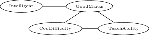
Markov Networks

• If all the potential are strictly positive, we can use a log-linear model (where the \(f_i\)s are features)

\( \begin{array}{c} P(\mathbf{x})=\frac{\exp({\sum_i w_i f_i(\mathbf{x_i})})}{Z}\\ Z=\sum_{\mathbf{x}}\exp({\sum_i w_i f_i(\mathbf{x_i})}))\\ f_i(Intelligent, GoodMarks)=\left\{ \begin{array}{ll} 1 &\mbox{if $\neg$Intelligent$\vee$GoodMarks}\\ 0 & \mbox{otherwise} \end{array}\right.\\ w_i=1.5 \end{array}\)

Markov Logic

• A Markov Logic Network (MLN) [Richardson, Domingos ML06] is a set of pairs \((F, w)\) where \(F\) is a formula in first-order logic \(w\) is a real number

• Together with a set of constants, it defines a Markov network with

  • One node for each grounding of each predicate in the MLN

  • One feature for each grounding of each formula \(F\) in the MLN, with the corresponding weight \(w\)

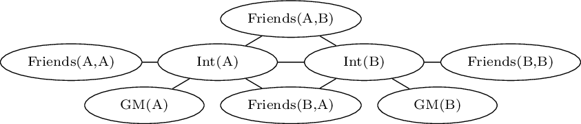
Markov Logic Example

\[\begin{array}{ll} 1.5 &\forall x\ Intelligent(x)\rightarrow GoodMarks(x)\\ 1.1&\forall x,y\ Friends(x,y)\rightarrow (Intelligent(x)\leftrightarrow Intelligent(y)) \end{array}\]

• Constants Anna (A) and Bob (B)

Markov Networks

• Probability of an interpretation \(\mathbf{x}\) \[P(\mathbf{x})=\frac{\exp({\sum_i w_i n_i(\mathbf{x_i})})}{Z}\]

• \(n_i(\mathbf{x_i})=\) number of true groundings of formula \(F_i\) in \(\mathbf{x}\)

• Typed variables and constants greatly reduce size of ground Markov net

Reasoning Tasks

• Inference: we want to compute the probability of a query given the model and, possibly, some evidence

• Weight learning: we know the structural part of the model (the logic formulas) but not the numeric part (the weights) and we want to infer the weights from data

• Structure learning we want to infer both the structure and the weights of the model from data

Applications

• Link prediction: given a (social) network, compute the probability of the existence of a link between two entities (UWCSE)

advisedby(X, Y) :0.7 :-
  publication(P, X),
  publication(P, Y),
  student(X).

Applications

• Classify web pages on the basis of the link structure (WebKB)

coursePage(Page1): 0.3 :- linkTo(Page2,Page1),coursePage(Page2).
coursePage(Page1): 0.6 :- linkTo(Page2,Page1),facultyPage(Page2).
...
coursePage(Page): 0.9 :- has('syllabus',Page).
...

Applications

• Entity resolution: identify identical entities in text or databases

samebib(A,B):0.9 :- 
    samebib(A,C), samebib(C,B).
sameauthor(A,B):0.6 :- 
  sameauthor(A,C), sameauthor(C,B).
sametitle(A,B):0.7 :- 
  sametitle(A,C), sametitle(C,B).
samevenue(A,B):0.65 :- 
  samevenue(A,C), samevenue(C,B).
samebib(B,C):0.5 :-
  author(B,D),author(C,E),sameauthor(D,E).
samebib(B,C):0.7 :-
  title(B,D),title(C,E),sametitle(D,E).
samebib(B,C):0.6 :-
  venue(B,D),venue(C,E),samevenue(D,E).
samevenue(B,C):0.3 :-
  haswordvenue(B,logic),
  haswordvenue(C,logic).
...

Applications

• Chemistry: given the chemical composition of a substance, predict its mutagenicity or its carcenogenicity

active(A):0.4 :-
   atm(A,B,c,29,C), 
   gteq(C,-0.003), 
   ring_size_5(A,D).
active(A):0.6:-
   lumo(A,B), lteq(B,-2.072).
active(A):0.3 :-
   bond(A,B,C,2), 
   bond(A,C,D,1), 
   ring_size_5(A,E).
active(A):0.7 :-
   carbon_6_ring(A,B).
active(A):0.8 :-
   anthracene(A,B).
...

Applications

• Medicine: diagnose diseases on the basis of patient information (Hepatitis), influence of genes on HIV, risk of falling of elderly people

Inference for PLP under DS

• Computing the probability of a query (no evidence)

• Knowledge compilation:

  • compile the program to an intermediate representation

    • Binary Decision Diagrams (BDD) (ProbLog [De Raedt et al. IJCAI07], cplint [Riguzzi AIIA07,Riguzzi LJIGPL09], PITA [Riguzzi & Swift ICLP10])

    • deterministic, Decomposable Negation Normal Form circuit (d-DNNF) (ProbLog2 [Fierens et al. TPLP15])

    • Sentential Decision Diagrams

  • compute the probability by weighted model counting

Inference for PLP under DS

• Bayesian Network based:

  • Convert to BN

  • Use BN inference algorithms (CVE [Meert et al. ILP09])

• Lifted inference

Knowledge Compilation

• Assign Boolean random variables to the probabilistic rules

• Given a query \(Q\), compute its explanations, assignments to the random variables that are sufficient for entailing the query

• Let \(K\) be the set of all possible explanations

• Build a Boolean formula \(F(Q)\)

• Build a BDD representing \(F(Q)\)

ProbLog

\[\begin{array}{l} sneezing(X)\leftarrow \mathit{flu}(X),\mathit{flu}\_sneezing(X).\\ sneezing(X)\leftarrow hay\_\mathit{fever}(X),hay\_\mathit{fever}\_sneezing(X).\\ \mathit{flu}(bob).\\ hay\_\mathit{fever}(bob).\\ 0.7::\mathit{flu}\_sneezing(X).\\ 0.8::hay\_\mathit{fever}\_sneezing(X).\\ \end{array}\]

Definitions

• Composite choice \(\kappa\): consistent set of atomic choices \((C_i,\theta_j,l)\) with \(l\in\{1,2\}\)

• Set of worlds compatible with \(\kappa\): \(\omega_\kappa=\{w_\sigma|\kappa \subseteq \sigma\}\)

• Explanation \(\kappa\) for a query \(Q\): \(Q\) is true in every world of \(\omega_\kappa\)

• A set of composite choices \(K\) is covering with respect to \(Q\): every world \(w\) in which \(Q\) is true is such that \(w\in\omega_K\) where \(\omega_K=\bigcup_{\kappa\in K}\omega_\kappa\)

• Example: \[\label{expls} K_1=\{\{(C_1,\{X/bob\},1)\},\{(C_2,\{X/bob\},1)\}\}\] is covering for \(sneezing(bob)\).

Finding Explanations

• All explanations for the query are collected

• ProbLog: source to source transformation for facts, use of dynamic database

• cplint (PITA): source to source transformation, addition of an argument to predicates

Explanation Based Inference Algorithm

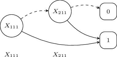
• \(K=\) set of explanations found for \(Q\), the probability of \(Q\) is given by the probability of the formula \[f_K(\mathbf{X})=\bigvee_{\kappa\in K}\bigwedge_{(C_i,\theta_j,l)\in\kappa}(X_{C_i\theta_j}=l)\] where \(X_{C_i\theta_j}\) is a random variable whose domain is \({1,2}\) and \(P(X_{C_i\theta_j}=l)=P_0(C_i,l)\)

• Binary domain: we use a Boolean variable \(X_{ij}\) to represent \((X_{C_i\theta_j}=1)\)

• \(\overline{X_{ij}}\) represents \((X_{C_i\theta_j}=2)\)

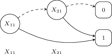
Example

A set of covering explanations for \( sneezing(bob) \) is \(K=\{\kappa_1,\kappa_2\}\)

\(\kappa_1=\{(C_1,\{X/bob\},1)\}\)   \(\kappa_2=\{(C_2,\{X/bob\},1)\}\)

\(K=\{\kappa_1,\kappa_2\}\)

\(f_{K}(\mathbf{X})=(X_{C_1\{X/bob\}}=1)\vee (X_{C_2\{X/bob\}}=1)\).

\(X_{11}=(X_{C_1\{X/bob\}}=1)\)    \(X_{21}=(X_{C_2\{X/bob\}}=1)\)

\(f_{K}(\mathbf{X})=X_{11}\vee X_{21}\).

\(P(f_{K}(\mathbf{X}))=P(X_{11}\vee X_{21})=P(X_{11})+P(X_{21})-P(X_{11})P(X_{21})\)

• In order to compute the probability, we must make the explanations mutually exclusive

•  [De Raedt at. IJCAI07]: Binary Decision Diagram (BDD)

Binary Decision Diagrams

• A BDD for a function of Boolean variables is a rooted graph that has one level for each Boolean variable

• A node \(n\) in a BDD has two children: one corresponding to the 1 value of the variable associated with \(n\) and one corresponding the 0 value of the variable

• The leaves store either 0 or 1.

Binary Decision Diagrams

• BDDs can be built by combining simpler BDDs using Boolean operators

• While building BDDs, simplification operations can be applied that delete or merge nodes

• Merging is performed when the diagram contains two identical sub-diagrams

• Deletion is performed when both arcs from a node point to the same node

• A reduced BDD often has a much smaller number of nodes with respect to the original BDD

Binary Decision Diagrams

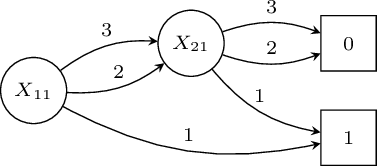
\[f_K(\mathbf{X})=X_{11}\times f_K^{X_{11}}(\mathbf{X})+\neg X_{11}\times f_K^{\neg X_{11}}(\mathbf{X})\]

\[P(f_K(\mathbf{X}))=P(X_{11})P(f_K^{X_{11}}(\mathbf{X}))+(1-P(X_{11}))P(f_K^{\neg X_1}(\mathbf{X}))\]

\[P(f_K(\mathbf{X}))=0.7\cdot P(f_K^{X_{11}}(\mathbf{X}))+0.3\cdot P(f_K^{\neg X_{11}}(\mathbf{X}))\]

Probability from a BDD

• Dynamic programming algorithm [De Raedt et al IJCAI07]

• Initialize map \(p\)

• Call \(\mathrm{Prob}(root)\)

• Function \(\mathrm{Prob}(n)\)

• if \(p(n)\) exists, return \(p(n)\)

• if \(n\) is a terminal note

  • return \(value(n)\)

• else

  • \(prob:=\mathrm{Prob}(child_1(n)\times p(v(n))+\mathrm{Prob}(child_0(n))\times (1-p(v(n)))\)

  • Add \((n,prob)\) to \(p\), return \(prob\)

Logic Programs with Annotated Disjunctions

\[\begin{array}{llll} C_1=&strong\_sneezing(X):0.3\vee moderate\_sneezing(X):0.5&\leftarrow& flu(X).\\ C_2=&strong\_sneezing(X):0.2\vee moderate\_sneezing(X):0.6&\leftarrow& hay\_fever(X).\\ C_3=&flu(bob).\\ C_4=&hay\_fever(bob).\\ \end{array}\]

• Distributions over the head of rules

• More than two head atoms

Example

A set of covering explanations for \( strong\_sneezing(bob) \) is \(K=\{\kappa_1,\kappa_2\}\)

\(\kappa_1=\{(C_1,\{X/bob\},1)\}\)

\(\kappa_2=\{(C_2,\{X/bob\},1)\}\)

\(K=\{\kappa_1,\kappa_2\}\)

\(X_{11}=X_{C_1\{X/bob\}}\)

\(X_{21}=X_{C_2\{X/bob\}}\)

\(f_{K}(\mathbf{X})=(X_{11}=1)\vee (X_{21}=1)\).

\(P(f_{X})=P(X_{11}=1)+P(X_{21}=1)-P(X_{11}=1)P(X_{21}=1)\)

• To make the explanations mutually exclusive: Multivalued Decision Diagram (MDD)

Multivalued Decision Diagrams

\[f_K(\mathbf{X})=\bigvee_{l \in|X_{11}|}(X_{11}=l)\wedge f_K^{X_{11}=l}(\mathbf{X})\]

\[P(f_K(\mathbf{X}))=\sum_{l \in|X_{11}|}P(X_{11}=l)P(f_K^{X_{11}=l}(\mathbf{X}))\]

\[f_K(\mathbf{X})=(X_{11}=1)\wedge f_K^{X_{11}=1}(\mathbf{X})+(X_{11}=2)\wedge f_K^{X_{11}=2}(\mathbf{X})+(X_{11}=3)\wedge f_K^{X_{11}=3}(\mathbf{X})\]

\[f_K(\mathbf{X})=0.3\cdot P(f_K^{X_{11}=1}(\mathbf{X}))+0.5\cdot P(f_K^{X_{11}=2}(\mathbf{X}))+0.2\cdot P(f_K^{X_{11}=3}(\mathbf{X}))\]

Manipulating Multivalued Decision Diagrams

• Use an MDD package

• Convert to BDD, use a BDD package: BDD packages more developed, more efficient

• Conversion to BDD

  • Log encoding

  • Binary splits: more efficient

Transformation to a Binary Decision Diagram

• For a variable \(X_{ij}\) having \(n\) values, we use \(n-1\) Boolean variables \(X_{ij1},\ldots,X_{ijn-1}\)

• \(X_{ij}=l\) for \(l=1,\ldots n-1\): \(\overline{X_{ij1}}\wedge\overline{X_{ij2}}\wedge\ldots \wedge \overline{X_{ijl-1}}\wedge X_{ijl}\),

• \(X_{ij}=n\): \(\overline{X_{ij1}}\wedge\overline{X_{ij2}}\wedge\ldots \wedge\overline{X_{ijn-1}}\).

• Parameters: \(P(X_{ij1})=P(X_{ij}=1)\ldots P(X_{ijl})=\frac{P(X_{ij}=l)}{\prod_{m=1}^{l-1}(1-P(X_{ijm}))}\).

Approximate Inference

• Inference problem is #P hard

• For large models inference is intractable

• Approximate inference

  • Monte Carlo: draw samples of the truth value of the query

  • Iterative deepening: gives a lower and an upper bound

  • Compute only the best \(k\) explanations: branch and bound, gives a lower bound

Monte Carlo

• The disjunctive clause

  \(C_r=H_1:\alpha_1\vee \ldots\vee H_n:\alpha_n\leftarrow L_1,\ldots,L_m.\)

  is transformed into the set of clauses \(MC(C_r)\)

  \(\begin{array}{l} MC(C_r,1)=H_1\leftarrow L_1,\ldots,L_m,sample\_head(n,r,VC,NH),NH=1.\\ \ldots\\ MC(C_r,n)=H_n\leftarrow L_1,\ldots,L_m,sample\_head(n,r,VC,NH),NH=n.\\ \end{array}\)

• Sample truth value of query Q:

  ...
    (call(Q)->    NT1 is NT+1 ;   NT1 =NT),
  ...

Inference in DISPONTE

• The probability of a query \(Q\) can be computed according to the distribution semantics by first finding the explanations for \(Q\) in the knowledge base

• Explanation: subset of axioms of the KB that is sufficient for entailing \(Q\)

• All the explanations for \(Q\) must be found, corresponding to all ways of proving \(Q\)

Inference in DISPONTE

• Probability of \(Q\) \(\rightarrow\) probability of the DNF formula \[F(Q)= \bigvee_{e\in E_Q} ( \bigwedge_{F_i \in e} X_{i} )\] where \(E_Q\) is the set of explanations and \(X_i\) is a Boolean random variable associated to axiom \(F_i\)

• Binary Decision Diagrams for efficiently computing the probability of the DNF formula

Example

\[\begin{aligned} &&E_1=0.4::{\mathit{fluffy}}: Cat\\ &&E_2=0.3::tom : Cat\\ &&E_3=0.6:: Cat \sqsubseteq Pet\\ &&\exists hasAnimal.Pet \sqsubseteq NatureLover\\ &&(kevin, {\mathit{fluffy}}):hasAnimal \\ &&(kevin, tom):hasAnimal \end{aligned}\]

• \(Q=kevin:NatureLover\) has two explanations:
  

  { (\(E_1\)), (\(E_3\)) }
  { (\(E_2\)), (\(E_3\)) }

• \(P(Q)=0.4\times 0.6 \times(1-0.3) + 0.3 \times 0.6 =0.348\)

BUNDLE

• Binary decision diagrams for Uncertain reasoNing on Description Logic thEories [Riguzzi et al. SWJ15]

• BUNDLE performs inference over DISPONTE knowledge bases.

• It exploits an underlying ontology reasoner able to return all explanations for a query, such as Pellet [Sirin et al, WS 2007]

• Then DNF formula built and converted to BDDs for computing the probability

TRILL

• Tableau Reasoner for descrIption Logics in proLog

• TRILL implements the tableau algorithm using Prolog

• It resolves the axiom pinpointing problem in which we are interested in the set of explanations that entail a query

• It returns the set of the explanations

• It can build BDDs encoding the set of explanations and return the probability

TRILL

• Available online at http://trill.lamping.unife.it/

• Pets example http://trill.lamping.unife.it/trill_on_swish/example/peoplePets.owl

Parameter Learning

• Problem: given a set of interpretations, a program, find the parameters maximizing the likelihood of the interpretations (or of instances of a target predicate)

• The interpretations record the truth value of ground atoms, not of the choice variables

• Unseen data: relative frequency can’t be used

Parameter Learning

• An Expectation-Maximization algorithm must be used:

  • Expectation step: the distribution of the unseen variables in each instance is computed given the observed data

  • Maximization step: new parameters are computed from the distributions using relative frequency

  • End when likelihood does not improve anymore

Parameter Learning

•  [Thon et al. ECML 2008] proposed an adaptation of EM for CPT-L, a simplified version of LPADs

•  The algorithm computes the counts efficiently by repeatedly traversing the BDDs representing the explanations

•  [Ishihata et al. ILP 2008] independently proposed a similar algorithm

• LFI-ProbLog [Gutamnn et al. ECML 2011]: EM for ProbLog

• EMBLEM [Riguzzi & Bellodi IDA 2013] adapts [Ishihata et al. ILP 2008] to LPADs

EMBLEM

• EM over Bdds for probabilistic Logic programs Efficient Mining

• Input: an LPAD; logical interpretations (data); target predicate(s)

• all ground atoms in the interpretations for the target predicate(s) correspond to as many queries

• BDDs encode the explanations for each query \(Q\)

• Expectations computed with two passes over the BDDs

EDGE

• Em over bDds for description loGics paramEter learning

• EDGE is inspired to EMBLEM [Bellodi and Riguzzi, IDA 2013]

• Takes as input a DL theory and a number of examples that represent queries.

• The queries are concept assertions and are divided into:

  1. positive examples;

  2. negative examples.

• EDGE computes the explanations of each example using BUNDLE, that builds the corresponding BDD.

  • For negative examples, EDGE computes the explanations of the query, builds the BDD and then negates it.

Structure Learning for LPADs

• Given a trivial LPAD or an empty one, a set of interpretations (data)

• Find the model and the parameters that maximize the probability of the data (log-likelihood)

• SLIPCOVER: Structure LearnIng of Probabilistic logic program by searching OVER the clause space EMBLEM [Riguzzi & Bellodi TPLP 2015]

  1. Beam search in the space of clauses to find the promising ones

  2. Greedy search in the space of probabilistic programs guided by the LL of the data.

• Parameter learning by means of EMBLEM

SLIPCOVER

• Cycle on the set of predicates that can appear in the head of clauses, either target or background

• For each predicate, beam search in the space of clauses

• The initial set of beams is generated by building a set of bottom clauses as in Progol [Muggleton NGC 1995]

Mode Declarations

• Syntax

modeh(RecallNumber,PredicateMode).
modeb(RecallNumber,PredicateMode).

• RecallNumber can be a number or *. Usually *. Maximum number of answers to queries to include in the bottom clause

• PredicateMode: template of the form:

p(ModeType, ModeType,...) 

Mode Declarations

• ModeType can be:

  • Simple:

    • +T input variables of type T;

    • -T output variables of type T; or

    • #T, -#T constants of type T.

  • Structured: of the form f(..) where f is a function symbol and every argument can be either simple or structured.

Mode Declarations

• Some examples:

modeb(1,mem(+number,+list)). 
modeb(1,dec(+integer,-integer)). 
modeb(1,mult(+integer,+integer,-integer)). 
modeb(1,plus(+integer,+integer,-integer)). 
modeb(1,(+integer)=(#integer)). 
modeb(*,has_car(+train,-car))
modeb(1,mem(+number,[+number|+list])). 

Bottom Clause \(\bot\)

• Most specific clause covering an example \(e\)

• Form: \(e\leftarrow B\)

• \(B\): set of ground literals that are true regarding the example \(e\)

• \(B\) obtained by considering the constants in \(e\) and querying the predicates of the background for true atoms regarding these constants

• A map from types to lists of constants is kept, it is enlarged with constants in the answers to the queries and the procedure is iterated a user-defined number of times

• Values for output arguments are used as input arguments for other predicates

Bottom Clause \(\bot\)

• Initialize to empty a map \(m\) from types to lists of values

• Pick a \(modeh(r,s)\), an example \(e\) matching \(s\), add to \(m(T)\) the values of \(+T\) arguments in \(e\)

• For \(i=1\) to \(d\)

  • For each \(modeb(r,s)\)

Bottom Clause \(\bot\)

• For each possible way of building a query \(q\) from \(s\) by replacing \(+T\) and \(\#T\) arguments with constants from \(m(T)\) and all other arguments with variables

  • Find all possible answers for \(q\) and put them in a list \(L\)

  • \(L':=\) \(r\) elements sampled from \(L\)

  • For each \(l\in L'\), add the values in \(l\) corresponding to \(-T\) or \(-\#T\) to \(m(T)\)

Bottom Clause \(\bot\)

• Example:

\(e=father(john,mary)\)

\(B=\{parent(john,mary), parent(david,steve),\)

\(parent(kathy,mary), female(kathy),male(john), male(david)\}\)

\(modeh(father(+person,+person)).\)

\(modeb(parent(+person,-person)).\)    \(modeb(parent(-\#person,+person)).\)

\(modeb(male(+person)).\)   \(modeb(female(\#person)).\)

\(e\leftarrow B=father(john,mary)\leftarrow parent(john,mary),male(john),\)

\(parent(kathy,mary),female(kathy).\)

Bottom Clause \(\bot\)

• The resulting ground clause \(\bot\) is then processed by replacing each term in a + or - placemarker with a variable

• An input variable (+T) must appear as an output variable with the same type in a previous literal and a constant (#T or -#T) is not replaced by a variable.

\(\bot=father(X,Y)\leftarrow parent(X,Y),male(X),parent(kathy,Y),female(kathy).\)

SLIPCOVER

• The initial beam associated with predicate \(P/Ar\) will contain the clause with the empty body \(h:0.5.\) for each bottom clause \(h\ {:\!-}\ b_1,\ldots,b_m\)

• In each iteration of the cycle over predicates, it performs a beam search in the space of clauses for the predicate.

• The beam contains couples \((Cl, LIterals)\) where \(Literals=\{b_1,\ldots,b_m\}\)

• For each clause \(Cl\) of the form \(Head \ {:\!-}\ Body\), the refinements are computed by adding a literal from \(Literals\) to the body.

SLIPCOVER

• The tuple (\(Cl'\), \(Literals'\)) indicates a refined clause \(Cl'\) together with the new set \(Literals'\)

• EMBLEM is then executed for a theory composed of the single refined clause.

• LL is used as the score of the updated clause \((Cl'',Literals')\).

• \((Cl'',Literals')\) is then inserted into a list of promising clauses.

• Two lists are used, \(TC\) for target predicates and \(BC\) for background predicates.

• These lists ave a maximum size

SLIPCOVER

• After the clause search phase, SLIPCOVER performs a greedy search in the space of theories:

  • it starts with an empty theory and adds a target clause at a time from the list \(TC\).

  • After each addition, it runs EMBLEM and computes the LL of the data as the score of the resulting theory.

  • If the score is better than the current best, the clause is kept in the theory, otherwise it is discarded.

• Finally, SLIPCOVER adds all the clauses in \(BC\) to the theory and performs parameter learning on the resulting theory.

Experiments - Area Under the PR Curve

Experiments - Area Under the PR Curve

Bongard Problems

• Introduced by the Russian scientist M. Bongard

• Pictures, some positive and some negative

• Problem: discriminate between the two classes.

• The pictures contain shapes with different properties, such as small, large, pointing down, … and different relationships between them, such as inside, above, …

Input File

Preamble

:-use_module(library(slipcover)).
:- if(current_predicate(use_rendering/1)).
:- use_rendering(c3).
:- use_rendering(lpad).
:- endif.
:-sc.
:- set_sc(megaex_bottom,20).
:- set_sc(max_iter,3).
:- set_sc(max_iter_structure,10).
:- set_sc(maxdepth_var,4).
:- set_sc(verbosity,1).

See http://cplint.lamping.unife.it/help/help-cplint.html for a list of options

Input File

Theory for parameter learning and background

bg([]).
in([
(pos:0.5 :-
    circle(A),
    in(B,A)),
(pos:0.5 :-
    circle(A),
    triangle(B))]).

Input File

Data: two formats, models

begin(model(2)).
pos.
triangle(o5).
config(o5,up).
square(o4).
in(o4,o5).
circle(o3).
triangle(o2).
config(o2,up).
in(o2,o3).
triangle(o1).
config(o1,up).
end(model(2)).

begin(model(3)).
neg(pos).
circle(o4).
circle(o3).
in(o3,o4).
....

Input File

Data: two formats, keys (internal representation)

pos(2).
triangle(2,o5).
config(2,o5,up).
square(2,o4).
in(2,o4,o5).
circle(2,o3).
triangle(2,o2).
config(2,o2,up).
in(2,o2,o3).
triangle(2,o1).
config(2,o1,up).

neg(pos(3)).
circle(3,o4).
circle(3,o3).
in(3,o3,o4).
square(3,o2).
circle(3,o1).
in(3,o1,o2).
....

Input File

• Folds

• Target predicates: output(<predicate>)

• Input predicates are those whose atoms you are not interested in predicting

  input_cw(<predicate>/<arity>).

  True atoms are those in the interpretations and those derivable from them using the background knowledge

• Open world input predicates are declared with

  input(<predicate>/<arity>).

  the facts in the interpretations, the background clauses and the clauses of the input program are used to derive atoms

Input File

fold(train,[2,3,5,...]).
fold(test,[490,491,494,...]).
output(pos/0).
input_cw(triangle/1).
input_cw(square/1).
input_cw(circle/1).
input_cw(in/2).
input_cw(config/2).

Input File

• Language bias

• \(determination(p/n,q/m)\): atoms for \(q/m\) can appear in the body of rules for \(p/n\)

determination(pos/0,triangle/1).
determination(pos/0,square/1).
determination(pos/0,circle/1).
determination(pos/0,in/2).
determination(pos/0,config/2).
modeh(*,pos).
modeb(*,triangle(-obj)).
modeb(*,square(-obj)).
modeb(*,circle(-obj)).
modeb(*,in(+obj,-obj)).
modeb(*,in(-obj,+obj)).
modeb(*,config(+obj,-#dir)).

Input File

Search bias

lookahead(logp(B),[(B=_C)]).

Bongard Problems

• Parameter learning

induce_par([train],P),
  test(P,[test],LL,AUCROC,ROC,AUCPR,PR).

• Structure learning

induce([train],P),
  test(P,[test],LL,AUCROC,ROC,AUCPR,PR).

Exercise

Write SLIPCOVER input file for

• University Database http://www.cs.sfu.ca/~oschulte/jbn/dataset.html Data university.pl

• Mutagenesis http://www.doc.ic.ac.uk/~shm/mutagenesis.html Data muta.pl

Conclusions

• Exciting field!

• Much is left to do:

  • Lifted inference

  • Continuous variables

  • Structure learning search strategies

References

• Bellodi, E. and Riguzzi, F. (2012). Learning the structure of probabilistic logic programs. In Inductive Logic Programming 21st International Conference, ILP 2011, London, UK, July 31 - August 3, 2011. Revised Papers, volume 7207 of LNCS, pages 61-75, Heidelberg, Germany. Springer.

• Bellodi, E. and Riguzzi, F. (2013). Expectation Maximization over binary decision diagrams for probabilistic logic programs. Intelligent Data Analysis, 17(2).

• Breese, J. S., Goldman, R. P., and Wellman, M. P. (1994). Introduction to the special section on knowledge-based construction of probabilistic and decision models. IEEE Transactions On Systems, Man and Cybernetics, 24(11):1577-1579.

References

• Dantsin, E. (1991). Probabilistic logic programs and their semantics. In Russian Conference on Logic Programming, volume 592 of LNCS, pages 152-164. Springer.

• De Raedt, L., Kimmig, A., and Toivonen, H. (2007). Problog: A probabilistic prolog and its application in link discovery. In International Joint Conference on Artificial Intelligence, pages 2462-2467.

• Fierens, D., den Broeck, G.V., Renkens, J., Shterionov, D.S., Gutmann, B., Thon, I., Janssens, G., De Raedt, L.: Inference and learning in probabilistic logic pro- grams using weighted boolean formulas. Theory and Practice of Logic Program- ming 15(3), 358-401 (2015)

References

• Gutmann, B., Thon, I., and Raedt, L. D. (2011). Learning the parameters of probabilistic logic programs from interpretations. In European Conference on Machine Learning and Knowledge Discovery in Databases, volume 6911 of LNCS, pages 581-596. Springer.

• Ishihata, M., Kameya, Y., Sato, T., and Minato, S. (2008). Propositionalizing the em algorithm by bdds. In Late Breaking Papers of the 18th International Conf. on Inductive Logic Programming, pages 44-49.

• Meert, W., Struyf, J., and Blockeel, H. (2009). CP-Logic theory inference with contextual variable elimination and comparison to bdd based inference methods. In ILP 2009.

References

• Meert, W., Taghipour, N., and Blockeel, H. (2010). First-order bayes-ball. In Balcázar, J. L., Bonchi, F., Gionis, A., and Sebag, M., editors, Machine Learning and Knowledge Discovery in Databases, European Conference, ECML PKDD 2010, Barcelona, Spain, September 20-24, 2010, Proceedings, Part II, volume 6322 of Lecture Notes in Computer Science, pages 369-384. Springer.

• Muggleton, S. (1995). Inverse entailment and progol. New Generation Comput., 13(3&4):245-286.

• Poole, D. (1993). Logic programming, abduction and probability - a top-down anytime algorithm for estimating prior and posterior probabilities. New Gener. Comput., 11(3):377-400.

• Poole, D. (1997). The Independent Choice Logic for modelling multiple agents under uncertainty. Artif. Intell., 94(1-2):7-56.

References

• Riguzzi, F. (2007). A top down interpreter for LPAD and CP-logic. In Congress of the Italian Association for Artificial Intelligence, number 4733 in LNAI, pages 109-120. Springer.

• Riguzzi, F. (2009). Extended semantics and inference for the Independent Choice Logic. Logic Journal of the IGPL.

• Riguzzi, F. and Swift, T. (2010). Tabling and Answer Subsumption for Reasoning on Logic Programs with Annotated Disjunctions. In Hermenegildo, M. and Schaub, T., editors, Technical Communications of the 26th Int’l. Conference on Logic Programming (ICLP10), volume 7 of Leibniz International Proceedings in Informatics (LIPIcs), pages 162-171, Dagstuhl, Germany. Schloss Dagstuhl-Leibniz-Zentrum fuer Informatik.

References

• Sato, T. (1995). A statistical learning method for logic programs with distribution semantics. In International Conference on Logic Programming, pages 715-729.

• Shachter, R. D. (1998). Bayes-ball: The rational pastime (for determining irrelevance and requisite information in belief networks and influence diagrams. In In Uncertainty in Artificial Intelligence, pages 480-487. Morgan Kaufmann.

• Thon, I., Landwehr, N., and Raedt, L. D. (2008). A simple model for sequences of relational state descriptions. In Daelemans, W., Goethals, B., and Morik, K., editors, Machine Learning and Knowledge Discovery in Databases, European Conference, ECML/PKDD 2008, Antwerp, Belgium, September 15-19, 2008, Proceedings, Part II, volume 5212 of Lecture Notes in Computer Science, pages 506-521. Springer.

References

• Vennekens, J., Verbaeten, S., and Bruynooghe, M. (2004). Logic programs with annotated disjunctions. In International Conference on Logic Programming, volume 3131 of LNCS, pages 195-209. Springer.

• Breese, J. S., Goldman, R. P., and Wellman, M. P. (1994). Introduction to the special section on knowledge-based construction of probabilistic and decision models. IEEE Transactions On Systems, Man and Cybernetics, 24(11):1577-1579.

• Costa, Vitor Santos, et al. CLP(BN): Constraint logic programming for probabilistic knowledge. Proceedings of the Nineteenth conference on Uncertainty in Artificial Intelligence. Morgan Kaufmann Publishers Inc., 2002.

• Richardson, Matthew, and Pedro Domingos. Markov logic networks. Machine learning 62.1-2 (2006): 107-136.

References

• Riguzzi, Fabrizio, et al. “Probabilistic description logics under the distribution semantics.” Semantic Web 6.5 (2015): 477-501.